Basic Usage of dust_mie

Single Particle Size Evaluation

Here is how to evaluate the Mie coefficients for Quartz at 1.0 microns with a particle size of 0.5 microns.

from dust_mie import calc_mie
qext, qsca, qback, g = calc_mie.get_mie_coeff(wav=2.0,r=1.0,material='SiO2')

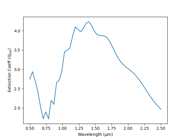
Or, here’s how to show the extinction as a function of wavelength:

from dust_mie import calc_mie
import numpy as np
import matplotlib.pyplot as plt

wave = np.linspace(0.5,2.5,50)
qext, qsca, qback, g = calc_mie.get_mie_coeff(wave,r=1.0,material='SiO2')

plt.plot(wave,qext)
plt.xlabel('Wavelength ($\mu$m)')
plt.ylabel('Extinction Coeff (Q$_{ext}$)')
plt.savefig('extinct_func.png')

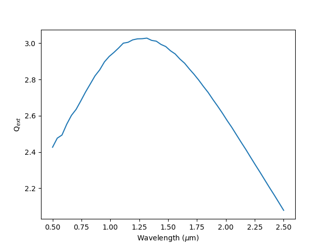
Particle Size Distribution Evaluation

You can also calculate the extinction function for a log-normal particle size distribution. Here, the sigma of the distribution is set to be 0.5

from dust_mie import calc_mie
import numpy as np
import matplotlib.pyplot as plt

wave = np.linspace(0.5,2.5,50)
qext, qsca, qback, g = calc_mie.get_mie_coeff_distribution(wave,r=1.0,material='SiO2',s=0.5)

plt.plot(wave,qext)
plt.xlabel('Wavelength ($\mu$m)')
plt.ylabel('Q$_{ext}$')
plt.savefig('extinct_func_distribution.png')

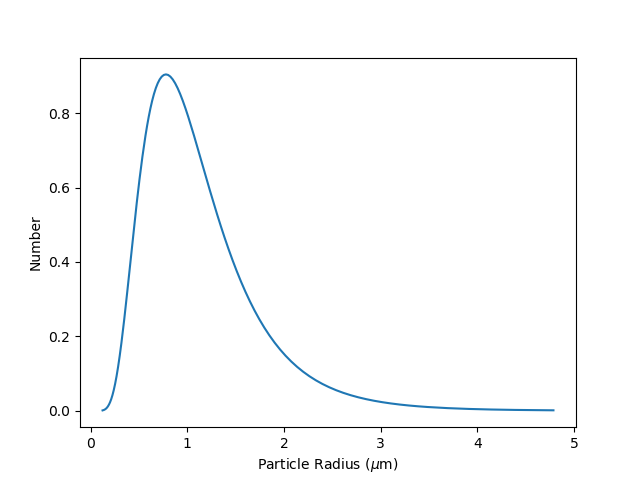
Plot the Particle Size Distribution

You can plot the particle size distribution for a log-normal function.

from dust_mie import calc_mie
import matplotlib.pyplot as plt

median_r = 1.0
s = 0.5

r, dr = calc_mie.get_r_to_evaluate(r=median_r,s=s)

n = calc_mie.lognorm(r,s=s,med=median_r)

plt.plot(r,n)
plt.xlabel('Particle Radius ($\mu$m)')
plt.ylabel('Number')
plt.savefig('radius_distribution.png')